Kernel Methods

Kernel methods are a class of algorithms used for pattern analysis, where the data is transformed into a higher-dimensional space to make it easier to classify or analyze. The kernel trick is particularly useful for algorithms that rely on dot products (e.g., Support Vector Machines), allowing them to operate in higher-dimensional spaces

Types of Kernels

• Linear Kernel: No transformation used when data is linearly separable.
• Polynomial Kernel: Maps the input space into a higher degree polynomial space.
• Radial Basis Function (RBF) Kernel: Maps the input into an infinite-dimensional space

Scaling and Standardization

Scaling and standardization are preprocessing techniques used to normalize data, especially for algorithms sensitive to feature magnitudes (like K-NN or SVM).

Scaling

Scaling refers to bringing all the features into a specific range, typically [0, 1] or [-1, 1]. This is important for distance-based algorithms like K-NN or SVM which depend on feature magnitudes. If one feature has a much larger range than others, it could dominate the distance calculation.

Formula

• x: The original value of the feature you want to scale
• min(x): The minimum value of that feature in your dataset.
• max(x): The maximum value of that feature in your dataset
• x′: The scaled value of xxx, now normalized between 0 and 1

Standardization

Center features around zero. Standardization transforms data such that:

• The mean of the transformed data becomes 0.
• The standard deviation becomes 1.

Formula

• X = Original value of the feature
• μ (mu) = Mean of the feature.
• σ (sigma) = Standard deviation of the feature.
• X standardized​ = Standardized value of XXX

Example

Mean /µ = (50+60+70+80+90)/5 = 70

Variance =

Calculate standard deviation (σ) = sqrt of 200​ ≈14.142

New values or Standardized values have a mean of zero and a standard deviation of 1. Any extremes have been standardized

Why Standardize Data?

• Ensures all features contribute equally.
• Makes different datasets or features comparable

K-Nearest Neighbors (K-NN)

• Model used when more than two classes
• It is a supervised machine learning method used for classification and regression tasks.
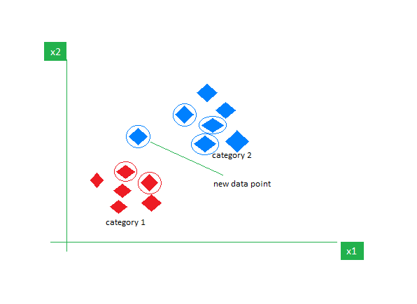
• It operates on the principle that data points with similar characteristics are likely to be in close proximity within the feature space.
• It assumes each new applicant is like previous applicant
• If K = 5, then the 5 nearest points to this new applicant are selected. Of these points if 3 are red, 1 is blue and 1 is green, new applicant is assumed to be Red
• Ideal value of K = 10

How Does KNN Work?

• Distance Metric: A distance function (such as Euclidean, Manhattan, or Minkowski distance) is used to measure the similarity between data points. The choice of distance metric can affect the performance of the algorithm.
• Selecting ‘K’ Neighbors: For a new data point that you want to classify or predict, the algorithm identifies the ‘K’ data points in the training set that are closest to it.
• Making a Decision:
  • Classification: The class of the new data point is determined by a majority vote among its K nearest neighbors.
  • Regression: The value of the new data point is predicted by averaging the values of its K nearest neighbors.
    1. Steps in Calculating KNN

Step 1: Selecting the optimal value of K

K represents the number of nearest neighbors that needs to be considered while making predictions.

Step 2: Calculating distance

To measure the similarity between target and training data points, Euclidean distance is used. Distance is calculated between each of the data points in the dataset and target point.

Step 3: Finding Nearest Neighbors

The k data points with the smallest distances to the target point are the nearest neighbors.

Step 4: Voting for Classification

• The class labels of K-nearest neighbors are determined by performing majority voting. The class with the most occurrences among the neighbors becomes the predicted class for the target data point.

1. Distance Metrics Used in KNN Algorithm

As we know that the KNN algorithm helps us identify the nearest points or the groups for a query point. But to determine the closest groups or the nearest points for a query point we need some metric. For this purpose, we use below distance metrics:

Euclidean Distance

This is nothing but the cartesian distance between the two points which are in the plane/hyperplane. Euclidean distance can also be visualized as the length of the straight line that joins the two points which are into consideration.

distance(x,Xi)=∑j=1d(xj–Xij)2]distance(x,Xi​)=∑j=1d​(xj​–Xij​​)2​]

• 1. When to use KNN

Ideal for dataset which require classification in more than two classes with two or more features